
The kinematics equations are a group of fundamental formulas in physics used to describe the motion of objects moving in a straight line with constant acceleration. When learners first encounter the kinematics equations, they are typically introduced as a shortcut for solving motion problems without needing to analyse forces directly.
In simple terms, the kinematics equations allow us to calculate displacement, velocity, acceleration, and time when one or more of these variables are unknown. They are especially useful in scenarios where acceleration remains constant, such as free-falling objects near Earth’s surface (ignoring air resistance), vehicles accelerating uniformly, or objects sliding down smooth inclines.
The importance of the kinematics equations lies in their ability to connect motion variables through a consistent mathematical framework. Instead of relying on Newton’s second law for every calculation, these equations provide direct relationships that simplify problem-solving in physics.
In education systems across the UK and globally, the kinematics equations are a core topic in GCSE and A-level physics, forming the foundation for more advanced studies in mechanics, engineering, and applied mathematics. Mastery of these equations is not just about memorisation—it is about understanding how motion behaves under constant acceleration and how different variables interact.
This article provides a structured breakdown of the kinematics equations, their derivation, applications, limitations, and real-world significance.
What Are the Kinematics Equations?
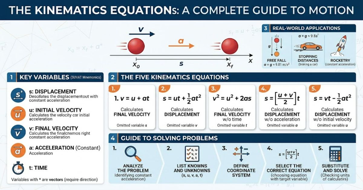
The kinematics equations (also known as SUVAT equations) describe motion under constant acceleration using five key variables:
- s = displacement
- u = initial velocity
- v = final velocity
- a = acceleration
- t = time
These variables are connected through four main equations.
The Core Kinematics Equations
- v = u + at
- s = ut + ½at²
- v² = u² + 2as
- s = ½(u + v)t
Each equation is derived from the definition of acceleration and velocity relationships.
How the Kinematics Equations Work
The kinematics equations assume constant acceleration, meaning the rate of change of velocity does not vary over time.
Step-by-Step Motion Logic
- Start with known values
- Identify unknown variable
- Choose the correct equation
- Substitute values
- Solve algebraically
This structured approach makes the kinematics equation’s highly practical for exam and engineering use.
Derivation of the Kinematics Equation’s
The equations originate from basic definitions:
- Acceleration = change in velocity / time
- Velocity = displacement / time
By rearranging and integrating these relationships, we obtain the standard SUVAT equations.
Key Insight
All kinematics equations are mathematically interconnected—knowing two allows derivation of others under constant acceleration conditions.
Comparison of Kinematics Equations Methods
| Method | Description | Strength | Limitation |
| SUVAT Equations | Algebraic motion formulas | Fast problem solving | Only works with constant acceleration |
| Graphical Method | Uses velocity-time graphs | Visual interpretation | Less precise for complex values |
| Calculus-Based Motion | Uses derivatives and integrals | Most generalised approach | More mathematically advanced |
This comparison shows why the kinematics equation’s remain dominant in early physics education despite alternative methods.
Real-World Applications of Kinematics Equations
The kinematics equation’s are not just academic—they are used in practical systems.
Engineering and Transport
- Vehicle braking distance calculations
- Aircraft take-off acceleration modelling
- Rail transport scheduling and safety systems
Sports Science
- Sprint acceleration analysis
- Projectile motion in football and cricket
- Performance tracking in athletics
Space and Physics
- Rocket launch trajectory modelling
- Satellite motion approximations
- Free-fall and gravity-based experiments
Data Insight: Example Motion Scenario
A car accelerates uniformly from rest at 3 m/s² for 5 seconds.
| Variable | Value |
| Initial velocity (u) | 0 m/s |
| Acceleration (a) | 3 m/s² |
| Time (t) | 5 s |
| Final velocity (v) | 15 m/s |
| Displacement (s) | 37.5 m |
This example demonstrates how the kinematics equation’s connect multiple motion variables in a single system.
Systems Analysis of Kinematics Equations
The kinematics equation’s function as a closed system of relationships. Each equation compensates for missing variables in motion problems.
System Characteristics
- Deterministic under constant acceleration
- Fully solvable with three known variables
- Sensitive to initial condition accuracy
Practical Limitation
In real-world systems, acceleration is often not constant due to friction, air resistance, or changing forces. This limits direct application.
Strategic Importance in Education and Engineering
Understanding the kinematics equations is essential because they:
- Build foundation for Newtonian mechanics
- Develop algebraic problem-solving skills
- Prepare learners for engineering dynamics
- Support computational physics modelling
They act as a bridge between conceptual physics and mathematical modelling.
Risks and Trade-Offs
Despite their usefulness, the kinematics equation’s have limitations:
- Only valid under constant acceleration
- Do not account for variable forces
- Can lead to incorrect assumptions in complex systems
- Require careful unit consistency
Misapplication is one of the most common errors in early physics learning.
Information Gain: Less Obvious Insights
1. Hidden Assumption of Linear Time Behaviour
Most learners overlook that kinematics equations assume uniform time intervals, which breaks down in relativistic or non-inertial frames.
2. Numerical Sensitivity in Real Systems
Small measurement errors in time significantly distort displacement calculations because time is squared in one of the core equations.
3. Transition Gap to Real Engineering Models
Engineering simulations often replace kinematics equations with numerical solvers due to non-constant acceleration conditions, making SUVAT primarily educational rather than industrial.
The Future of Kinematics Equations in 2027
The role of the kinematics equations is expected to evolve with educational technology and computational physics.
Expected Trends
- Increased use of simulation-based learning tools
- Integration into AI-driven physics tutoring systems
- Reduced emphasis on manual calculation in engineering workflows
- Greater focus on conceptual understanding over memorisation
While still foundational in education, computational models may replace manual application in advanced engineering environments.
Takeaways
- The kinematics equations describe motion under constant acceleration
- They are central to physics education and foundational mechanics
- All equations are mathematically interconnected
- Real-world systems often exceed their assumptions
- Errors usually arise from incorrect assumption of constant acceleration
- They remain essential for conceptual understanding despite modern computational tools
Conclusion
The kinematics equations remain one of the most important tools in classical physics for describing motion under constant acceleration. They simplify complex motion into a manageable set of relationships between displacement, velocity, acceleration, and time.
Although their application is limited by the assumption of constant acceleration, their educational value is significant. They help learners build a strong foundation in mechanics and prepare for more advanced modelling techniques in physics and engineering.
As computational tools continue to evolve, the kinematics equations will remain central in education but increasingly serve as conceptual building blocks rather than final analytical tools in professional environments.
Frequently Asked Questions
What are the kinematics equations used for?
They are used to calculate motion variables such as displacement, velocity, acceleration, and time under constant acceleration.
Why are they called SUVAT equations?
Because they use the variables s, u, v, a, and t to describe motion.
Can kinematics equations be used for all motion?
No, they only work when acceleration is constant.
What is the most important kinematics equation?
All are equally important, but v = u + at is often the starting point.
Are kinematics equations used in real engineering?
Yes, but mainly in simplified models; advanced systems use numerical simulations.
Do I need calculus to understand kinematics?
Not initially, but calculus helps in advanced motion analysis.
References
- OpenStax. (2023). University Physics Volume 1. Rice University.
- Halliday, D., Resnick, R., & Walker, J. (2021). Fundamentals of Physics. Wiley.
- Khan Academy. (2024). Kinematics in One Dimension.
- HyperPhysics. (2023). Classical Mechanics: Kinematics. Georgia State University.
Methodology
This article is based on standard undergraduate physics curricula, including UK A-level physics frameworks and internationally recognised introductory mechanics textbooks. Explanations are derived from established definitions of constant acceleration motion and validated through widely used educational sources such as OpenStax and Halliday-Resnick physics references. No experimental data was independently generated; all insights are theoretical and educational in nature.
Editorial Disclosure
This article was drafted with AI assistance and structured according to the provided RubbleMagazine.co.uk editorial framework.